|
|
| SECTION I - PROFILING |
| Mean Velocity (U) Definition |
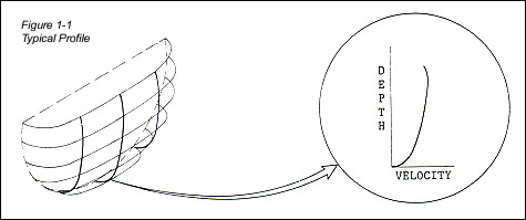
A particle of water near the
conduit wall will not move as fast as a particle toward the center. To understand this, we
need to look at the molecules of moving liquids. The first layer of molecules stick to the
wall of the conduit. The next layer will move by sliding across the first layer. This
happens throughout the flow with each successive layer moving at a faster velocity. The
change in velocity is greater mean the conduit wall than it is toward the center. If
velocity measurements of each layer could be taken, a velocity profile similar to the one
in Figure 1-1 would be produced. Notice that the velocity decreases near the surface
because of surface effects. Since most flows fit this profile, this is called the typical
profile. There are, however, situations which will cause other profile shapes and it is
usually more difficult to calculate flow with these shapes.
|
 |
To calculate flow, an average or mean of all the varying
velocities must be determined. Since it is not practical to measure the velocity of each
layer of molecules, methods have been developed with which a mean velocity (U) can be
determined from velocity measurements taken at various positions in the flow. |
|
|
|
| Cross-Sectional Area |
| The cross-sectional area of the
flow is determined from a level measurement and the channel shape. It is important that
the mean velocity measurement and the level measurement is done at the same location in
the channel. |
| Site Selection |
| A site that produces the typical
profile shape will give the most accurate results. In a majority of the cases, problem
sites can be identified by a visual inspection. Site inspection guidelines are as follows: |
- The channel should have as much straight run as possible.
Where the length of straight run is limited, the length upstream from the profile should
be twice the downstream length.
- The channel should be free of flow disturbances. Look for
protruding pipe joints, budden changes in diameter, contributing sidestreams, outgoing
sidestreams, or obstructions. Clean any rock, sediment, or other debris that might be on
the bottom of the pipe.
- The flow should be free of swirls, eddies, vortices, backward
flow, or dead zones. Be careful of areas that have visible swirls on the surface.
- Avoid areas immediately downstream from sharp bends or
obstructions.
- Avoid converging or diverging flow (approach to a flume) and
vertical drops.
- Avoid areas immediately downstream from a sluice gate or
there
the channel empties into a body of stationary water.
|
| Choosing The Method |
| All profiling methods can be used
in a site that produces a typical profile and has sufficient level to measure three point
velocities. If you cannot avoid sites with nontypical profiles or low flows, the following
guidelines will help in choosing a method that will give the best results. |
|
Low Flows - In flows of less than two inches, the 0.9 x Vmax
method is recommended.
Rapidly Changing Flows - A flow that is changing more than
10% in three minutes or less can be classified as rapidly changing. The 0.9 x Vmax or 0.4
methods take the least amount of time. However, these methods usually require a typical
profile shape for accurate results.
Asymmetrical Flow - There will be a difference of 30% or more
between the right and left side velocities in asymmetrical flow. The 2-D method is
recommended.
Vertical Drop (outfalls) - The 2-D method is recommended for
outfalls. Remember to measure the level on the same plane as the velocity profile.
Outfalls should be avoided wherever possible.
Nontypical Profile Shape -- If you suspect a profile shape
may not be typical, use the 2-D method.
Choosing the method will become easier as you gain
experience.
|
Profiling Checks |
For best possible results, you
should:
- Check the inside diameter of the conduit. Also measure the
horizontal and vertical diameters. If there is a difference, then average the diameter.
- Check for symmetry of flow.
- Check level several times furing the procedure.
- Check the invert for rocks, sediment, and other debris.
|
|
|
| Calculating U 0.9 x Vmax Method |
- Take a series of point velocity measurements throughout the
intire flow.
- Identify the fastest velocity. In most cases, this is usually
located in the center just beneath the surface.
- Multiply the fastest velocity by 0.9 for U.
|
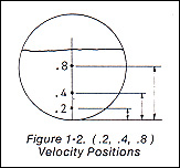
| Calculating U 0.2, 0.4, 0.8 of Depth
Method |
- Measure depth of flow
- Locate possitions on the centerline by: 0.2 x depth., 0.4 x
depth., 0.8 x depth
- At 0.2, 0.4 and 0.8 positions, measure and record the point
velocities (Fig. 1-2). In manmade channels, measure the 0.2, 0.4 and 0.8 positions from
the bottom.
- Average 0.2 and 0.8 velocities.
- Average the 0.4 velocity with the 0.2 and 0.8 average for U
|
|
|
|
|
| Calculating U 0.4 Method |
| A simplified version of the .2,
.4, .8 method is to measure the velocity at the .4 position and use this as U. This method
is probably the least accurate because it uses only one data point and assumes that a
typical profile exists. This is also called the 60% of depth methods. |
|
|
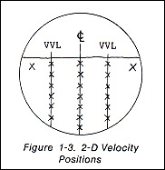
| Calculating U 2-D Method |
- Locate the centerline of the flow.
- Take at least seven velocity measurements at different depths
along the centerline.
- Average all measurements except outliers for U. Remember to
include the corner measurements.
|
- Locate vertical velocity lines
(VVL) halfway between the
centerline and the side smalls of the conduit. This is measured at the widest part of the
flow.
- Take velocity readings at different depths on the VVL. The
distance between those depths should be the same as those on the centerline.
- Take final point velocity readings
at the right and left
corners of the flow.
- Check the data for any outliers. If a best fit curve of the
velocity profile were plotted, an outlier would lie outside the best fit curve region.
|
|
|
| Calculating U VPT Method |
| The Velocity Profiling Technique
(VPT) was first described by N.T. Debevoise and R.B. Fernandez in the November 1984 issure
of the WPCF Journal. With this method, a series of point velocity measurements are taken
at different depths along the centerline of the flow. These measurements along with level
are input not a VPT computer program which calculates U and flow. The program and a
detailed description of this method is available from MMI. |
|
|
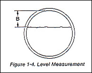
Measuring Level Circular Conduits
- Measure the inside diameter of the conduit.
- Measure distance B (Fig. 1-4)
- Subtract B from the inside diameter of the conduit for the
depth of flow. This eliminates the problem of the rules interfering with the liquid.
|
|
|
|
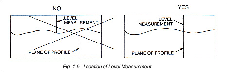
The level measurement and the velocity profile must be on
the same plane for proper application of the continuity equation.
|
 |
|
|
|
| SECTION II - CALCULATING FLOW |
| Circular Conduits |
To calculate flow in circular conduits you need:
- The mean velocity U from Section I
|
|
- The depth of flow at the time of profile.
- The inside diameter of the conduit
|
| Calculate level/diameter ratio by:
L ÷ D = L/D |
|
Where:
L is depth of flow in inches at time of profile
D is the inside diameter in inches.
L/D is level/diameter ratio |
| Where: K is flow unit multiplier. |
|
Find the appropriate L/D ratio in the L/D column and move to
the right to the K in the appropriate units column. |
| Calculate D² by: (Diameter Inches
÷
12)² |
|
Where: D² is diameter in feet squared.
This matches the velocity unit of ft/sec. |
| Calculate flow by: K x D² x U = flow |
|
Example: What is the flow in
millions of gallons per day of a
10-inch diameter conduit with a 6-inch level? The U has been calculated to be 1.5 ft/sec. |
| Calculate level/diameter ratio L/D: |
|
Level ratio L/D = 6 inches/10 inches = 0.6 |
| Identify K: |
|
K = 0.6 --> 0.3180 from Table II |
| Calculate D² |
|
D² = (10 in. ÷ 12
)² = (0.83 ft)² 0.6889 ft² |
| Calculate flow: K x D² x U = MGD |
|
0.3180 x 0.6889 ft² x 1.5 ft / sec =
0.328 MGD |
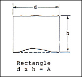
| Calculating Flow Rectangular Channel |
|
|
| Flow in rectangular channels is calculated by the following: |
|
- Determine U with the .2, .4, .8 method as described on above.
For large channel widths, use the .2, .6, .8 method as described on above for rivers and
streams. Velocity units must be in ft/sec.
- Calculate the cross-sectional area in ft²
by: [(Depth of Flow) in. ÷ 12] x [(Channel Width) in. ÷
12]
- Calculate flow by: U x (Cross-sectional area)
|
The result should be a flow rate in ft³
/sec. You can convert this to other flow units with the flow unit conversion multipliers
in attach. table. Example: What is the flow in a channel 24 inches wide with a 10-inch
flow?
| Solution: |
|
- Velocity measured at .2 = 1.5 ft / sec.
- U = (1.5 + 1.7 + 1.8) ÷ 3 = 1.67 ft/sec.
- From table 1 10 in. = 0.83 ft.
- Area = 0.83 ft x 2 ft = 1.66 ft²
- Flow = 1.67 ft² / sec. x 1.66 ft = 2.77 ft³
/ sec.
|
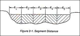
Calculating Flow Rivers and Streams
| Divide the width of the channel into a number of equal
segments with a distance "d" (Fig. 2-1). The more segments you use the better
the result. If the difference in mean velocity between two adjacent segments is greater
than 10%, the segments should be smaller. |
|
|
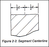
- Locate the center line for each segment at 1/2 d (Fig. 2-2)
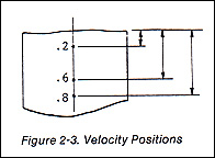
- Calculate .2, .6, .8 velocity position by:
- 0.2 x Depth.,
- 0.6 x Depth.,
- 0.8 x Depth.
- Measure the velocity at the 0.2, 0.6, and 0.8 positions.
|
|
|
| (NOTE) The 0.2,
0.6, and 0.8 positions for rivers and streams are measured from the surface. All depth and
velocity measurements must be on the same plane.
|
|
|
- Average the 0.2 and 0.8 velocities.
- Average the 0.6 velocity with the average of the 0.2 and 0.8
velocities for U.
- Calculate the flow of each segment by: (Segment Area) x U
- Sum the flow of the segments for total flow.
|
|
 |
 |
| Example: |
|
Convert 20 ft³ /sec (CFS) to millions of
gallons per day (MGD). |
| Solution: |
|
- Conversion factor = 0.64632.,
- 20 ft³ /sec x 0.64632 = 12.9264 MGD
|
Flow Units
| MGD -- Millions of Gallons per Day |
|
CMM -- Cubic Meters per Minute |
| GPM -- Gallons per Minute |
|
CMD -- Cubic Meters per Day |
| CFS -- Cubic Feet per Second |
|
LPM -- Liters per Minute |
|
|
|
